Multivariate Warping Models

In this research, we construct multivariate spatial models by deforming space. Through warping functions, nonstationary and asymmetric covariances on a geographical domain are modeled as simpler, more familiar, stationary and symmetric covariances on a warped domain.

Consider a bivariate spatial process $\Yvec(\svec) \equiv ( Y_1(\svec), Y_2(\svec))'$, $\svec \in G$, where we refer to $G \subset \mathbb{R}^2$ as the geographic domain. The cross-covariance functions are $$C_{ij,G}(\svec, \uvec) = \cov(Y_i(\svec), Y_j(\uvec)); \quad i,j = 1,2; \quad \svec, \uvec \in G,$$ where $\{ C_{ij,G}(\cdot \, , \cdot) \}$ are nonstationary and asymmetric (cross-)covariance functions. Under warping, they can expressed as simpler, usually stationary and symmetric (cross-)covariance functions, $\{ C_{ij,D}(\cdot \, , \cdot) \}$, on a deformed space $D$.

First, consider two warping functions $\fvec_1(\cdot), \fvec_2(\cdot)$ such that $\fvec_1, \fvec_2: G \to D$. In this case, $$\begin{equation*} C_{ij, G}(\svec, \uvec) = C_{ij, D}(\fvec_i(\svec), \fvec_j(\uvec)) = C^{o}_{ij, D}({\fvec_i(\svec) - \fvec_j(\uvec)}); \quad i,j = 1,2; \quad \svec,\uvec \in G, \end{equation*}$$ where $\{ C^{o}_{ij,D}(\cdot) \}$ are stationary and symmetric (cross-)covariance functions on the warped domain $D$.

In practice, any asymmetry present is likely to be simple and dominated by global shifts and rotations. To model asymmetry, we thus propose expressing each $\fvec_i(\cdot), i = 1,2$, as a composition of a shared warping function $\fvec(\cdot)$, and an aligning function $\gvec_i(\cdot)$. That is, for $i,j = 1,2$, we let $$\begin{align*} C_{ij, G}(\svec, \uvec) &= C_{ij, D}(\fvec \circ\gvec_i(\svec), \fvec \circ \gvec_j(\uvec)) \nonumber \\ &= C^{o}_{ij, D}(\fvec \circ \gvec_i(\svec) - \fvec \circ\gvec_j(\uvec)); \quad \svec,\uvec \in G. \end{align*}$$ We can choose the aligning functions $\gvec_i(\cdot), i = 1,2$, to be simple transformations that are commonly used to align spatial fields and which can include translations and rotations [@wiens2019surface], and the shared warping functions $\fvec(\cdot)$ to be composed of deep injective warping functions, which are able to introduce complex nonstationary behaviour (Zammit-Mangion et al. 2019).

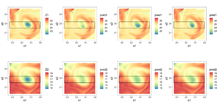
We applied the multivariate warping models on a dataset of ocean temperatures at two different depths. We analysed ocean temperatures at 0.5 metres depth and 318.1 metres depth on 1 July 2018 in the region 36.3$^{\circ}$N—39.6$^{\circ}$N and 60.0$^{\circ}$W—63.3$^{\circ}$W. Specifically, we considered 1600 observation locations in this region arranged on a $40 \times 40$ grid, but held-out data between 37.5$^{\circ}$N—38.2$^{\circ}$N to check the predictive performance of our model when data are missing in a large gap. We considered the following covariance models:

1. Model 1: A stationary, symmetric, parsimonious bivariate Matérn model (Gneiting, Kleiber, and Schlather 2010)

2. Model 2: A symmetric bivariate warping model, with the aligning functions as identity maps, with the warping function $\fvec(\cdot)$ a composition of axial warping units, a single-resolution radial basis function unit, and a Möbius transformation unit (see Zammit-Mangion et al. 2019 for a description of these units), with the parsimonious bivariate Matérn covariance model on the warped domain.

3. Model 3: An asymmetric bivariate warping model, with the aligning functions $\gvec_1(\cdot)$ an identity map, $\gvec_2(\cdot)$ an affine transformation, the warping function as in Model 2, with the parsimonious bivariate Matérn covariance model on the warped domain.

Figure 1 compares predictions obtained using Models 1—3 with each other. Note how Model 1 does not predict the low temperature anomaly as Models 2 and 3. Numeric results for the diagnostics are given in Table 1.

Figure 1: Comparison of predictions from Model 1, Model 2, and Model 3. Top row: Temperature at 0.5 metres, $Z_1$. Bottom row: Temperature at 318.1 metres, $Z_2$. From left to right: Observations, predictions from Model 1, Model 2, and Model 3. The rectangle depicts the hold-out region.

Table 1: Hold-out-validation results for the ocean temperatures at depths 0.5 meters and 318.1 meters, where data were missing in a block.

In this work we show that multivariate warping models can be used to efficiently capture nonstationarity and asymmetry present in multivariate spatial data. The multivariate spatial covariance models are relatively easy to fit, as they are built on a parsimonious set of warping functions, and are expressed in terms of models with stationary, symmetric, and possibly isotropic covariances on a warped domain. These models are shown to be able to provide better predictive performance than conventional stationary models, even when data are missing over large regions.

The code used in this work can be found at deepspat Github repository.

Most of the work described above can be found in the manuscript that is freely accessible at arXiv.

Authored by Q. Vu and A. Zammit-Mangion, 2020.